Trust Region Reflective Algorithm

The most relevant description of this algorithm can be found in the paper “A subspace, interior and conjugate gradient method for large-scale bound-constrained minimization problems” by Coleman and Li, some insights on its implementation can be found in MATLAB documentation here and here. The difficulty was that the algorithm incorporates several ideas, but it was not very clear how to combine them all together in the actual code. I will describe each idea separately and then outline the algorithm in general. I will consider the algorithm applied to a problem with known Hessian, in least squares we replace it by $J^T J$ . I won’t give any explanation or motivation for some things, if you are really interesting try digging into the original papers.

Interior Trust-Region Approach and Scaling Matrix

The minimization problem is stated as follows:

$\min f(x), \: x \in \mathcal{F} = \{x: l \leq x \leq u\}$

Some of the components of $l$ and $u$ can be infinite meaning no bound in this direction. Let’s use the notation $g(x) = \nabla f(x)$ and $H(x) = \nabla^2 f(x)$ . The first order necessary conditions for $x_*$ to be a local minimum:

$g(x_*)_i = 0 \text{ if } l_i < x_i < u_i$

$g(x_*)_i \leq 0 \text{ if } x_i = u_i$

$g(x_*)_i \geq 0 \text{ if } x_i = l_i$

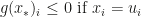
Define a vector $v(x)$ with the following components:

$v(x)_i = \begin{cases} u_i - x_i & g_i < 0 \text{ and } u_i < \infty \\ x_i - l_i & g_i > 0 \text{ and } l_i > -\infty \\ 1 & \text{otherwise} \end{cases}$

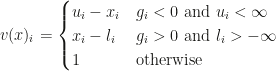
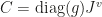
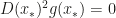
Its components are distances to the bounds at which anti-gradient points (if this distance is finite). Define a matrix $D(x) = \mathrm{diag}(v(x)^{1/2})$ , the first order optimality can be stated as $D(x_*)^2 g(x_*) = 0$ . Now we can think of our optimization problem as the diagonal system of nonlinear equations (I would say it is the main idea of this part):

$D^2(x) g(x) = 0$ .

The Jacobian of the left hand side exist whenever $v(x)_i \neq 0$ for all $i$ , which is true when $x \in \mathrm{int}(\mathcal{F})$ (not on the bound). Assume that this holds, then Newton step for this system satisfies:

$(D^2 H + \mathrm{diag}(g) J^v) p = - D^2 g$

Here $J_v$ is diagonal Jacobian matrix of $v(x)$ , its elements take values $\pm 1$ or $0$ , note that all elements of the matrix $C =\mathrm{diag}(g) J^v$ are non-negative. Now introduce the change of variables $x = D \hat{x}$ . In the new variables we have Newton step satisfying: $\hat{B} \hat{p} = -\hat{g}$ where $\hat{B} = D H D + C$ , $\hat{g} = D g$ (note that $\hat{g}$ is a proper gradient of $f$ with respect to “hat” variables). Looking at this Newton step we formulate corresponding trust-region problem:

$\displaystyle \min_{\hat{p}} \: \hat{m}(\hat{p}) = \frac{1}{2} \hat{p}^T B \hat{p} + \hat{g}^T \hat{p}, \text{ s. t. } \lVert \hat{p} \rVert \leq \Delta$ .

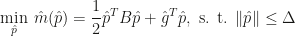
In the original space we have:

$B = H + D^{-1} C D^{-1}$ ,

and the equivalent trust-region problem

$\displaystyle \min_{p} \: m(p) = \frac{1}{2} p^T B p + g^T p, \text{ s. t. } \lVert D^{-1} p \rVert \leq \Delta$ .

From my experience the better approach is to solve the trust-region problem in “hat” space, so we don’t need to compute $D^{-1}$ which can become arbitrary large when the optimum is on the boundary and the algorithm approaches it.

A modified improvement ratio of out trust-region solution is computed as follows:

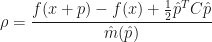
$\displaystyle \rho = \frac{f(x + p) - f(x) + \frac{1}{2}\hat{p}^T C \hat{p} } {\hat{m}(\hat{p})}$

Based on $\rho$ we adjust a radius of trust region using some reasonable strategy.

Now summary and conclusion for this section. Motivated by the first-order optimality condition we introduced a matrix $D$ and reformulated our problem as the system of nonlinear equations. Then motivated by the Newton process for this system we formulated the corresponding trust-region problem. The purpose of the matrix $D$ is to prevent steps directly into bounds, so that other variables can also be explored during the step. It absolutely doesn’t mean that after introducing such matrix we can ignore the bounds, specifically our estimates $x_k$ must remain strictly feasible. The full algorithm will be described below.

Reflective Transformation

This idea comes from another paper “On the convergence of reflective Newton methods for large-scale nonlinear minimization subject to bounds” by the same authors. Conceptually we apply a special transformation $x = R(y)$ , such that $y$ is unbounded variable and try to solve unconstrained problem $\min_y f(R(y))$ . The authors suggest a reflective transformation: a piecewise linear function, equal to identity when $y$ satisfies the initial bound constraints, otherwise reflected from the bounds as a beam of light (I hope you got the idea). I implemented it as follows (although don’t use this code anywhere):

import numpy as np

def reflective_transformation(y, l, u):
    if l is None:
        l = np.full_like(y, -np.inf)
    if u is None:
        u = np.full_like(y, np.inf)

    l_fin = np.isfinite(l)
    u_fin = np.isfinite(u)

    x = y.copy()

    m = l_fin & ~u_fin
    x[m] = np.maximum(y[m], 2 * l[m] - y[m])

    m = ~l_fin & u_fin
    x[m] = np.minimum(y[m], 2 * u[m] - y[m])

    m = l_fin & u_fin
    d = u - l
    t = np.remainder(y[m] - l[m], 2 * d[m])
    x[m] = l[m] + np.minimum(t, 2 * d[m] - t)

    return x

This transformation is simple and doesn’t significantly increase the complexity of the function to minimize. But it is not differentiable when $x$ is on the bounds, thus we again use strictly feasible iterates. The general idea of the reflective Newton method is to do line search along the reflective path (or a traditional straight line in $y$ space). According to the authors this method has cool properties, but it is used very modestly in the final large-scale Trust Region Reflective.

Large Scale Trust-Region Problem

In the previous post I conceptually described how to accurately solve trust-region subproblems arising in least-squares minimization. Here I again focus on least-squares setting and briefly describe how it can be solved approximately in large-scale.

Steihaug Conjugate Gradient. Apply conjugate gradient method to the normal equation until the current approximate solution falls outside the trust region (or indefinite direction is found if $J$ is rank deficient). This actually might be just the best approach for least squares as we don’t have negative curvature directions in $J^T J$ , and the only criticism of Steihaug-CG I read is that it can terminate before finding the negative curvature direction. I would assume that it is not very important for positive semidefinite case.
Two-dimensional subspace minimization. We form a basis consisting of two “good” vectors, then solve two-dimensional trust region problem with the exact method. The first vector is a gradient, the second is an approximate solution of linear least squares with the current $J$ (computed by LSQR or LSMR). When Jacobian is rank deficient the situation is somewhat problematic, as I noticed in this case a least-norm solution is useless for approximating a trust-region solution. In this case we need to add (not too big) regularization diagonal term to $J^T J$ . A recipe for this situation is given in “Approximate solution of the trust region problem by minimization over two-dimensional subspaces”.

Outline of Trust Region Reflective

Here is the high level description.

Consider the trust-region problem in “hat” space as described in the first section.
Find its solution by whatever method is appropriate (exact for small problems, approximate for large scale). Compute the corresponding solution in the original space $p = D \hat{p}$ .
Restrict this trust-region step to lie within bounds if necessary. Step back from the bounds by $\theta = \min(0.05, \lVert D^2 g \rVert)$ times the step length. Do it for all type of steps below.
Consider a single reflection of the trust-region step if bound was encountered in 3. Use 1-d minimization of the quadratic model to find the minimum along the reflected direction (this is trivial).
Find the minimum of the quadratic model along the $\hat{g}$ . (Rarely it can be better than the trust-region step because of the bounds.)
Choose the best step among 3, 4, 5. Compute the corresponding step in the original space as in 2, update $x$ .
Update the trust region radius by computing $\rho$ as described in the first section.
Check for convergence and go to 1 if the algorithm has not converged.

In the next two posts I will describe another type of algorithm which we call “dogbox” and provide comparison benchmark results.

4 thoughts on “Trust Region Reflective Algorithm”

Nathan Zimmerman says:

October 27, 2016 at 3:11 am

Many thanks for your work. You are the only person i’m aware of that has attempted to explain the trust region reflective problem. Is your implementation the one that is currently used in scipy?

LikeLike

1. nickmayorov says:
  
  November 17, 2016 at 6:49 pm
  
  I’m glad that it is useful for you.
  
  > Is your implementation the one that is currently used in scipy?
  
  Yes, it’s one of the algorithms available in scipy.optimize.least_squares
  
  Feel free to ask any questions you might have. I will try to check this blog from time to time.
  
  LikeLike
  
  1. Nathan Zimmerman says:
    
    November 20, 2016 at 2:21 am
    
    Yes it was very helpful. Much more readable than academic papers. I’ve been attempting to do bounded least squares and this was the algorithm matlab uses so I was trying to learn it. However, when I carefully made my own implementation based upon this post, it seemed this algorithm was far overkill for bounded least squares.
    The trust regions and reflection steps didn’t seem to be necessary. Perhaps if it was a bounded nonlinear function it would be necessary but not in the linear case. For a small scale case( n,m<100), a step of the following seemed to be fine:
    p = -(D^2 * H + diag(g) * Jv)^(-1) * D^2 * g
    So far for me, simply iterating based on these steps converged for a bounded least square problem generally in ~10 iterations. Prior to this, I was implementing an active set method that freezed the active bounds. However, this method was incredibly slow since only 1-2 bound could be identified per iteration and there may be 100s of active bounds.
    I needed a javascript solution hence me investigating my own solver since I wasn't aware of an existing bounded least squares JS implementation. Anyhow, heres my simplified implementation based off your implementation: https://github.com/NateZimmer/Maths.js/blob/master/Solvers/lsqBounds.js
    
    LikeLike
  2. nickmayorov says:
    
    November 26, 2016 at 11:38 pm
    
    Yes, the full algorithm is necessary only for non-linear problems. The concept of a trust-region doesn’t really makes sense for a linear problem.
    
    In fact I implemented also a solver for liner least squares with bounds, scipy.optimize.lsq_linear One of the algorithms it includes is a modification of trust-region-reflective (OK, “trust-region” is just a conventional name to make an analogy). Another one is a more well known “Bounded-Variable Least-Squares algorithm” (you can easily find a paper). It is more of a combinatorial algorithm and it doesn’t scale well for high dimensional problems, but for small problems is very good (it converges in a fixed number of steps in a very straightforward manner). So you might want to check that, implementation is available in scipy.
    
    LikeLike

GSOC 2015

by Nikolay Mayorov